Technical Report (version: 2015-09-12)
Abstract
The Ruby gem spitzy is a collection of methods for differential equations written in Ruby. Apart from an interface with the DASPK Fortran library there currently does not seem to exist another differential equation solver gem for Ruby. Currently, in its early development phase, spitzy has multiple methods to solve initial and boundary value ODEs, 2D Poisson's equation and the 1D advection equation. We present all currently implemented numerical schemes, their underlying theory and implementation details, as well as usage examples.
Table of Contents
Introduction
Under the project name spitzy, we are developing a collection of methods for differential equations written in the programming language Ruby. The idea to develop a Ruby differential equations library has its origin in the fact that apart from an interface with the DASPK Fortran library there currently does not seem to exist another differential equation solver gem for Ruby, even though a feature rich linear algebra library is available with NMatrix and a number of Ruby tools for scientific computing and visualisation are under active development by the Ruby Science Foundation (or SciRuby).
Currently spitzy includes the methods Dormand-Prince, forward Euler and second-order Adams-Bashforth for initial value problems, the numerical schemes Upwind, Lax-Friedrichs, Leapfrog and Lax-Wendroff for the one-dimensional linear advection equation, the five-point Laplacian method for the two-dimensional Poisson's equation, and the linear finite element Galerkin method for two-point boundary value problems.
In the following, we introduce the types of differential equations covered by the currently implemented methods, and present usage examples for the methods, as well as the underlying theory and implementation details.
Origin of the Name

Spitzy is this cute Pomeranian. Spitzy reads backwards as YZTIPS, which translates into:
Your Zappy-Tappy Initial and boundary value Partial (and ordinary) differential equation Solver
Installation
See github repository for instructions.
Initial Value Problems
An initial value problem is an ordinary differential equation of the form
- ODE: $\frac{dy}{dx} = f(x,y)$ for $a \leq x \leq b$,
- with initial condition $y(a) = y_0$.
For this kind of differential equation spitzy provides the class Spitzy::Ode, which currently has three methods, Dormand-Prince, Forward Euler and an Adams-Bashforth method of order 2.
Dormand-Prince
Dormand-Prince (or DOPRI, or RKDP) is an explicit method for solving initial value problems that automatically performs an error estimation and adapts the step size accordingly in order to keep the error of the numerical solution below a pre specified tolerance level. It was first introduced by Dormand and Prince in [DP80].
It is a member of the Runge-Kutta family of methods. In general, a Runge-Kutta method has the form $$u\subscript{n+1} = u\subscript{n} + h \sum\subscript{1}^s b\subscript{i}K\subscript{i},$$ where each $K\subscript{i}$ is an evaluation of the right hand side $f$ of the ODE at a specifically defined input value (for more detail, see section 11.8 in [QSS07]), and $s$ is called the number of stages of the Runge-Kutta method. The Dormand-Prince method has seven stages, but due to clever computational tricks it uses only six function evaluations. The last evaluated stage of a step of the algorithm is the same function evaluation as the first stage of the next step of the algorithm.
The Dormand-Prince method computes a fourth-order and a fifth-order approximations to the solution, and takes their difference as an estimate of the local truncation error of the forth-order scheme. Consequently, the estimated error is compared to a pre specified tolerance, and depending on the outcome of this comparison the step size is adjusted.
The method owes its computational efficiency to the fact that the utilized forth-order and fifth-order schemes share the same values $K\subscript{i}$.
As the numerical solution $u\subscript{n+1}$, which initializes the numerical scheme at the time step $n+2$, the method uses the fifth-order approximation. So, the method is fifth-order, as a whole.
Dormand-Prince is widely agreed on to be the go-to method for most ordinary differential equations (e.g. see [Sha86]). For example it is currently the default in MATLAB's ode45 solver, which is suggested as the first method to try by the MATLAB documentation.
Implementation
The Dormand-Prince method is implemented in the class Spitzy::Ode in spitzy. It can be utilized by setting the parameter method to :dopri when defining an Spitzy::Ode object.
When we apply the Dormand-Prince method, we need to specify the range of $x$ values, the initial condition, the maximal step size that we don't want the method to exceed, and the function $f(x,y)$ (as a Proc object or a supplied block). Optionally, we can specify the tolerance level for the error of the obtained numerical solution (the default is 0.01), and the maximal number of iterations for the algorithm (the default is 1e6). Since Dormand-Prince adjusts the step sizes according to an error estimate, the algorithm might require multiple iterations to evaluate the solution at one step, that is, the algorithm will keep on carrying out iterations until it finds a suitable step size (thus opening the door to never ending loops). That is the reason why the maximal number of iterations is a input parameter.
Examples
Let's look at an example. We consider the initial value problem:
- ODE: $\frac{dy}{dx} = 1 + \frac{y}{x} + \left(\frac{y}{x}\right)^2$, $1 \leq x \leq 4$,
- IC: $y(1) = 0$.
The following Ruby code computes a numerical solution to the above ODE using the Dormand-Prince method with a maximal step size of 0.1 in spitzy:
require 'spitzy'
f = proc { |t,y| 1.0 + y/t + (y/t)**2 }
dopri_sol = Spitzy::Ode.new(xrange: [1.0,4.0], dx: 0.1, yini: 0.0, &f)
If additionally we want to set the error tolerance to 1e-6 and the maximal number of performed iterations to 1e6, we can do:
dopri_sol = Spitzy::Ode.new(xrange: [1.0,4.0], dx: 0.1, yini: 0.0,
                    tol: 1e-6, maxiter: 1e6, &f)
The exact solution to the ODE is $y(x) = x\tan(\log(x))$.
We can now plot the obtained numerical solution and the exact solution with any Ruby visualization tool of our choice. Using the Ruby gem gnuplot we produce the figure shown below. One can clearly see that the Dormand-Prince solution agrees with the exact solution.
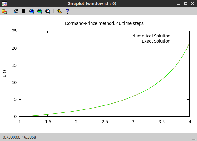
Using the exact solution, we can compute the error of the numerical solution. We can print further information about the obtained solution to the screen, using some of the attribute readers of Spitzy::Ode.

In particular, we see that the error of the numerical solution stays below the prescribed tolerance level, as intended.
Example: Automatic step size adjustment
We look at a second example that demonstrates the automatic step size adjustment capabilities of the Dormand-Prince method. Suppose we have the initial value problem:
- ODE: $\frac{dy}{dx} = -2y + e^{-2(x-6)^2}$, $0 \leq x \leq 10$,
- IC: $y(0) = 1$.
We apply the Dormand-Prince method with error tolerance 1e-6:
f = proc { |t,y| -2.0 * y + Math::exp(-2.0 * (t - 6.0)**2) }
dopri_sol = Spitzy::Ode.new(xrange: [0.0,10.0], dx: 1.5, yini: 1.0,
                    tol: 1e-6, maxiter: 1e6, &f)
and plot the obtained solution on the grid generated by the method:
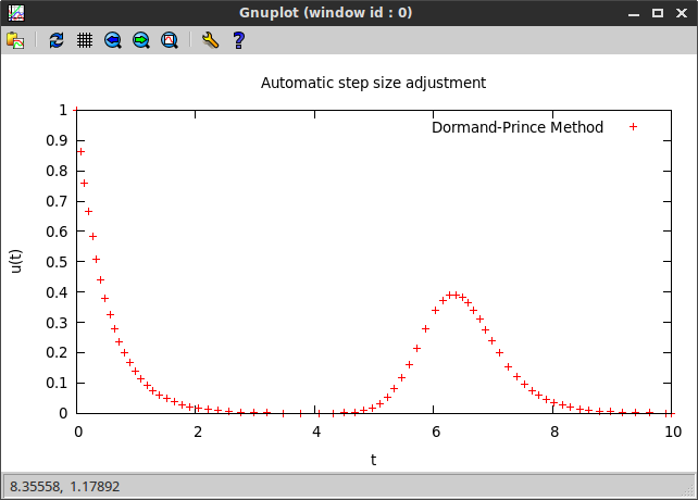
One can clearly see that the step size decreases in regions of bigger change in the slope of the function.
Forward Euler
The forward Euler method is the most basic method for solving ordinary differential equations. It is a first-order Runge-Kutta method, given by the explicit formula $$u\subscript{n+1} = u\subscript{n} + h f(x\subscript{n}, u\subscript{n}),$$ where $x\subscript{0}, x\subscript{1}, \ldots, x\subscript{N}$ are equally spaced grid points with spacing $h$ on the interval $[a,b]$. It is the most basic explicit method and often serves as a basis to construct more complex methods.
Implementation
The forward Euler method is implemented in the class Spitzy::Ode in spitzy. It can be utilized by setting the parameter method to :euler when defining an Spitzy::Ode object. When we apply the method, we need to specify the range of $x$ values, the initial condition, the step size for the $x$-grid, and the function $f(x,y)$ (as a Proc object or a supplied block).
In its implementation in spitzy, unlike the Dormand-Prince method, the forward Euler method cannot automatically control the step size or estimate the error of the obtained numerical solution.
Examples
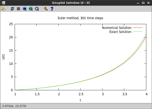
We apply the Euler method to the same differential equation as in the Dormand-Prince example above, namely:
- ODE: $\frac{dy}{dx} = 1 + \frac{y}{x} + \left(\frac{y}{x}\right)^2$, $1 \leq x \leq 4$,
- IC: $y(1) = 0$.
Using spitzy the following code computes the solution for this initial value problem.
f = proc { |t,y| 1.0 + y/t + (y/t)**2 }
euler_sol = Spitzy::Ode.new(xrange: [1.0,4.0], dx: 0.01,
                    yini: 0.0, method: :euler, &f)
If we plot the obtained numerical solution, we can see that, even though the Euler method evaluates the solution at a much finer grid, it performs much worse than the Dormand-Prince method. Nevertheless, there possibly are situations in which the simple Euler method is preferred over the rather complex Dormand-Prince.
Second-Order Adams-Bashforth
The Adams-Bashforth method implemented in spitzy is a second order method from the family of multi-step methods.
It is given by the explicit formula,
$$u\subscript{n+1} = u\subscript{n} + \frac{h}{2}(3f(x\subscript{n},u\subscript{n}) - f(x\subscript{n-1},u\subscript{n-1})).$$
One can derive this method by matching the Taylor expansions of the right- and the left-hand side of the equation
$$\frac{y\subscript{n+1} - y\subscript{n}}{h} = b\subscript{0} f(x\subscript{n},y\subscript{n}) + b\subscript{1} f(x\subscript{n-1},y\subscript{n-1}).$$
Implementation
The second-order Adams-Bashforth method is implemented in the class Spitzy::Ode in spitzy. It can be utilized by setting the parameter method to :ab2 when defining an Spitzy::Ode object.
As the Euler method, the Adams-Bashforth implementation in spitzy operates on a fixed pre specified step size, and takes as inputs the range of $x$ values, the initial condition, the step size for the $x$-grid, and the function $f(x,y)$ (as a Proc object or a supplied block).
Since the Adams-Bashforth method requires the last two functional values for the approximation of the next functional value, and since only one initial value is given, we apply Heun's method to approximate the functional value at the second time step. Heun's method is given by the following formula $$u\subscript{n+1} = u\subscript{n} + \frac{h}{2}(f(x\subscript{n},u\subscript{n}) + f(x\subscript{n+1}, u\subscript{n} + hf(x\subscript{n},u\subscript{n}))).$$ Heun's method is a Runge-Kutta method of order 2 (e.g. see exercise 1 from section 11.12 in [QSS07]). Thus, one application of Heun's method does not reduce the order of the successive application of the Adam-Bashforth method of order 2.
Example
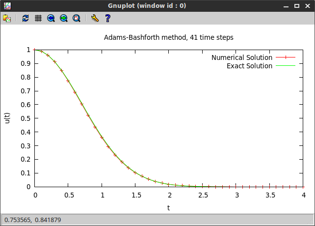
We demonstrate the Adams-Bashforth method by solving the following differential equation:
- ODE: $\frac{dy}{dx} = -2xy$, $0 \leq x \leq 4$,
- IC: $y(0) = 1$.
The implemented Adams-Bashforth scheme is a method of order two, which means that the error of the numerical solution is proportional to the square of the step size. Consequently, if we halve the step size, then the error of the numerical solution should reduce by a factor of four. We check this theoretical property by computing two solutions with step sizes 0.1 and 0.05, and comparing their errors (the exact solution is $y(x) = e^{-x^2}$. The following short code carries out the calculation, and its output is shown below.
require 'spitzy'

f = proc { |t,y| -2.0*t*y }
ab2_sol1 = Spitzy::Ode.new(xrange: [0.0,4.0], dx: 0.1,
                  yini: 1.0, method: :ab2, &f)
ab2_sol2 = Spitzy::Ode.new(xrange: [0.0,4.0], dx: 0.05,
                   yini: 1.0, method: :ab2, &f)

exact_sol1 = ab2_sol1.x.map { |tt| Math::exp(-(tt**2)) }
maxerror1 = exact_sol1.each_with_index.map {|n,i| n - ab2_sol1.u[i] }.max.abs
exact_sol2 = ab2_sol2.x.map { |tt| Math::exp(-(tt**2)) }
maxerror2 = exact_sol2.each_with_index.map {|n,i| n - ab2_sol2.u[i] }.max.abs

puts "Number of x steps: #{ab2_sol1.mx} and #{ab2_sol2.mx}"
puts "Error: #{maxerror1} and #{maxerror2}"
puts "Error ratio: #{maxerror1/maxerror2}"

As expected the error ratio is close to 4.
We also plot the numerical and the exact solutions.
Two-point Boundary Value Problems
A two-point boundary value problem that can be solved with 'spitzy' is an ordinary differential equation of the following general form:
- ODE: $-(\alpha u')'(x) + (\beta u')(x) + (\gamma u)(x) = f(x)$, for $a < x < b$,
- where $\alpha$, $\beta$ and $\gamma$ are constants or continuous functions of $x$ on $[a,b]$,
- with Dirichlet boundary conditions: $u(a) = u\subscript{a}$ and $u(b) = u\subscript{b}$.
Currently the linear finite element Galerkin method is the only scheme implemented in spitzy to solve this problem.
Linear Finite Element Galerkin
This section is largely based on section 12.4 in [QSS07]. The interested reader is referred there for a more rigorous presentation of what follows.
Background
Consider an ordinary differential equation of the following general form:
- ODE: $-(\alpha u')'(x) + (\beta u')(x) + (\gamma u)(x) = f(x)$, for $a < x < b$,
- where $\alpha$, $\beta$ and $\gamma$ are continuous functions of $x$ on $[a,b]$,
- with Dirichlet boundary conditions: $u(a) = u\subscript{a}$ and $u(b) = u\subscript{b}$.
We are looking for a weak solution to this problem, that is, a function $u$ that satisfies the integral equation $$\underset{[a,b]}{\int} \alpha u' v' dx + \underset{[a,b]}{\int} \beta u' v dx + \underset{[a,b]}{\int} \gamma u v dx = \underset{[a,b]}{\int} f v dx,$$ for every $v$ in the so-called test-function space $V$, which basically contains functions that have square-integrable distributional derivatives and vanish on the boundary of the domain of the ODE. If $u$ is a solution to the original formulation of the ODE then it also satisfies to integral formulation. However, a solution $u$ of the integral equation might not be twice differentiable.
Galerkin Method
The Galerkin method approximates $V$ with a finite dimensional functional space $V\subscript{h}$, which leads to a finite number of test functions $v$ that need to be tested against $u$ with the above integral equation. We denote the basis functions of $V\subscript{h}$ by $\phi\subscript{1}, \phi\subscript{2}, \ldots, \phi\subscript{N}$. Moreover, if we assume that $u$ also lies in the space $V\subscript{h}$, then the problem reduces to a linear system $$A\vec{u} = \vec{f},$$ where $A$ has entries $$a\subscript{ij} = \underset{[a,b]}{\int} \alpha \phi\subscript{i}' \phi\subscript{j}' dx + \underset{[a,b]}{\int} \beta \phi\subscript{i}' \phi\subscript{j} dx + \underset{[a,b]}{\int} \gamma \phi\subscript{i} \phi\subscript{j} dx,$$ and the right hand side vector $\vec{f}$ has entries $$f\subscript{i} = \underset{[a,b]}{\int} \alpha f' \phi\subscript{i}' dx + \underset{[a,b]}{\int} \beta f' \phi\subscript{i} dx + \underset{[a,b]}{\int} \gamma f \phi\subscript{i} dx.$$
The structure of $A$ and the degree of accuracy of the numerical solution depend on the form of the basis functions $\phi\subscript{1}, \phi\subscript{2}, \ldots, \phi\subscript{N}$, that is, on the choice of $V\subscript{h}$.
Finite Element Method
The finite element method chooses $V_h$ to be the space of continuous piecewise polynomials which are defined on subintervals of $[a, b]$ and vanish at $a$ and $b$.
Here, we only consider polynomials of degree 1, that is, continuous piecewise linear functions. Given an equally spaced grid $a = x\subscript{0} < x\subscript{1} < \ldots < x\subscript{n-1} < x\subscript{n} = b$, define for $i=1,2,\ldots,n-1$ the function $\phi\subscript{i}$ to be the continuous piecewise linear function that is equal to 1 at the node $x\subscript{i}$ and 0 at all other nodes. Thus, the basis functions have the following shape (the red line represents a linear combination of the basis functions):

Implementation
The linear finite element Galerkin method is implemented in class Spitzy::Bvp of the Ruby gem spitzy. It takes as inputs the interval of $x$ values as well as the Dirichlet boundary conditions at the two edges of the interval, the desired number of equally spaced grid points on which the numerical solution will be evaluated, and the functions $\alpha(x)$, $\beta(x)$, $\gamma(x)$ and $f(x)$ as Proc objects (or as Numeric if the function is constant).
The linear finite element Galerkin method boils down to a linear system
$A\vec{u} = \vec{f}$, where the matrix $A$ is tridiagonal. Currently, the Ruby implementation in spitzy uses the #solve method from the NMatrix gem.
However, the memory usage as well as the speed of the algorithm can be improved, as soon as pull request #301, which implements a #solve_tridiagonal method, is merged into the project.
Examples
Now let's look at some examples.
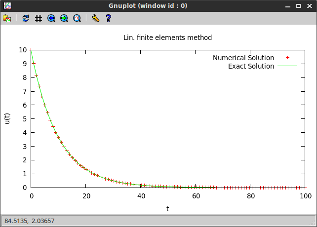
Example 1. Constant coefficients
First we look at example, where $\alpha$, $\beta$ and $\gamma$ are constants independent of $x$:
- ODE: $-800\pi u'' + 8\pi u = 0$, $0 < x < 100$,
- BC: $u(0) = 10$, $u(100) = \frac{10}{\cosh(10)}$.
We compute the numerical solution:
require 'spitzy'
bvp_sol = Spitzy::Bvp.new(xrange: [0.0, 100.0], mx: 100, bc: [10.0, 0.00090799859],
                  a: 800.0*Math::PI, b: 0.0, c: 8.0*Math::PI, f: 0.0)
The exact solution is $$u(x) = 10 \frac{\cosh\left(\frac{100 - x}{10}\right)}{\cosh(10)}.$$
We compare the obtained numerical to the exact solution by plotting both using the Ruby gnuplot gem:
Example 2. Non-constant coefficients
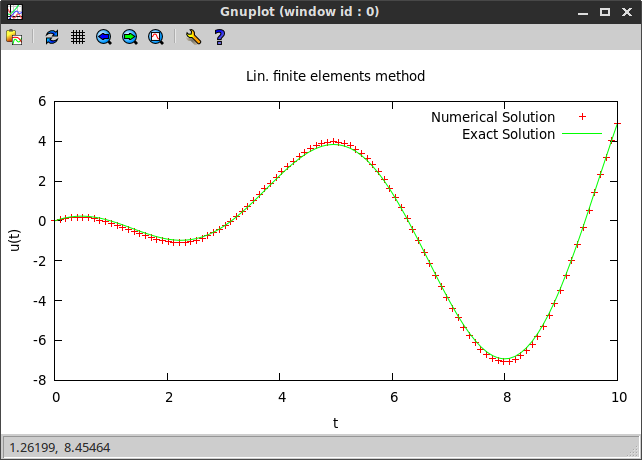
Now, let's consider an example where $\alpha$, $\beta$, $\gamma$ and $f$ are all functions of $x$.
- ODE: $-\frac{d}{dx}(-\cos(x)u'(x)) + \sin(x)u'(x) + \cos(x) u(x) = -2\cos^2(x)$, $0 < x < 10$,
- BC: $u(0) = 0$, $u(10) = -9\sin(10)$.
We use spitzy to compute the numerical solution:
a = Proc.new { |x| -Math::cos(x) }
b = Proc.new { |x| Math::sin(x) }
c = Proc.new { |x| Math::cos(x) }
f = Proc.new { |x| -2.0*(Math::cos(x))**2 }
xrange = [0.0, 10.0]
bc = [0.0, (1.0 - 10.0) * Math::sin(10.0)]
bvp_sol = Spitzy::Bvp.new(xrange: xrange, mx: 100, bc: bc,
                  a: a, b: b, c: c, f: f)
By taking derivatives one can check that the exact solution is given by $$u(x) = (1-x)\sin(x).$$
Again, we plot both, the numerical and the exact solution, and observe that they approximately agree.
2D Poisson's Equation
Poisson's equation is the elliptic boundary value problem:
- $\Delta u = f$ in $\Omega$,
- with the boundary condition: $u=g$ on $\partial \Omega$.
Here we only consider the 2-dimensional version of Poisson's problem, where $\Delta u = \frac{d^2 u}{dx^2} + \frac{d^2 u}{dy^2}$. We can discretized Poisson's equation by defining a mesh over the domain $\Omega$. If we denote by $\Omega\subscript{h}$ the set of the interior mesh points and by $\Gamma\subscript{h}$ the set of boundary mesh points, then the numerical solution needs to satisfy the discrete version of Poisson's problem written as:
- $\Delta\subscript{h} u = f$ in $\Omega\subscript{h}$,
- with the Dirichlet boundary condition: $u=g$ on $\Gamma\subscript{h}$.
Here $\Delta\subscript{h}$ is a consistent approximation of the operator $\Delta$, and it can be defined in various ways.
The only method currently implemented in spitzy defines the operator $\Delta\subscript{h}$ based on a five-point stencil, consisting of the point itself and its four immediate neighbors. We call it the five-point Laplacian method.
For more detail on the above and an introduction to various numerical methods for the solution of Poisson's equation we refer to [Arn11].
Five-point Laplacian
In the current implementation of the five-point Laplacian method we assume a rectangular domain, i.e. $\Omega = [a,b]\times[c,d]$, and that each side of the domain is subdivided into subintervals of the same length $h$.
Under such conditions the following approximation to the Laplacian operator can be used $$\Delta\subscript{h} u\subscript{i,j} = -\frac{1}{h^2} (4u\subscript{i,j} - u\subscript{i+1,j} - u\subscript{i-1,j} - u\subscript{i,j+1} - u\subscript{i,j-1}),$$ where $x\subscript{i,j}$ denotes the point in the discretization $\Omega\subscript{h}$ corresponding to the $i$th coordinate in $x$-direction and the $j$th coordinate in $y$-direction, and $u\subscript{i,j}$ is an approximation to the true solution $u(x\subscript{i,j})$. After a moment of reflection it is clear that this amounts to the second-order centered discretization of the second derivative in both, the $x$- and the $y$-directions.
It is an easy exercise to see that this problem reduces to the linear system
$$A\vec{u} = \vec{b},$$
where $\vec{u} = (u\subscript{1,1}, u\subscript{2,1}, \ldots, u\subscript{m,1}, \ldots, u\subscript{1,k}, u\subscript{2,k}, \dots, u\subscript{m,k}, \dots, u\subscript{1,n}, u\subscript{2,n}, \dots, u\subscript{m,n})^T$,
the matrix $A$ is pentadiagonal with constant values along each (sub-/super-)diagonal, and the right hand side $\vec{b}$ consists of values $f(x\subscript{i,j})$ with the boundary condition $g(x\subscript{i,j})$ subtracted when necessary. For more detail on the construction of $\vec{u}$, $A$ and $\vec{b}$ we refer to the definition of Spitzy::Bvp in the spitzy code.
It can be shown that the five-point Laplacian is a method of second order (see [Arn11]).
Implementation
The five-point Laplacian method is implemented in class Spitzy::PoissonsEq of the Ruby gem spitzy. It takes as inputs the rectangular domain in form of a range in $x$-direction and a range in $y$-directions, the step size $h$, the Dirichlet boundary condition as a function of $x$ and $y$, and the right hand side function $f(x,y)$ (each function is passed as a Proc object, or as Numeric if the function is constant).
A mesh grid is generated with the method #meshgrid from the NMatrix gem. Currently this method is available only in the development version of NMatrix.
Currently, the Ruby implementation in spitzy uses the #solve method from the NMatrix gem to solve the linear system.
Since the matrix $A$ is pentadiagonal other methods can significantly improve the computational speed as well as the memory usage. It would be straight forward to implement a modified successive over-relaxation method, which would only perform multiplications corresponding to the non-zero elements of $A$ (it would even be unnecessary to save the matrix at all, because all entries of $A$ are either $-4/h^2$, $1/h^2$ or $0$). However, such a method should probably be implemented in C, because it is questionable if it would beat NMatrix's #solve method (which is written in C) otherwise.
Examples
We test the five-point Laplacian method on the following partial differential equation:
- PDE: $\Delta u = e^{-\frac{x^2 + y^2}{2}} (x^2 + y^2 - 2)$,
- on the rectangular domain $[-1,1]\times[-5,5]$,
- with Dirichlet boundary conditions that agree with the exact solution $z = e^{-\frac{x^2 + y^2}{2}}$.
The numerical solution can be obtained with spitzy via the following three lines of code:
f = Proc.new { |x,y| Math::exp(-0.5*(x**2.0 + y**2.0)) * (x**2.0 + y**2.0 - 2.0) }
bc = Proc.new { |x,y| Math::exp(-0.5*(x**2.0 + y**2.0)) }
numsol = Spitzy::PoissonsEq.new(xrange: [-1.0,1.0], yrange: [-5.0, 5.0], h: 0.2, bc: bc, f: f)
We plot the numerical solution using the gnuplot Ruby gem, and the following code:
require 'gnuplot'
Gnuplot.open do |gp|
  Gnuplot::SPlot.new(gp) do |plot|
    plot.title "Five-point Laplacian method example"
    plot.xlabel "x"
    plot.ylabel "y"
    plot.zlabel "z"
    x = numsol.x.flatten
    y = numsol.y.flatten
    u = numsol.u.flatten
    plot.data << Gnuplot::DataSet.new([x,y,u]) do |ds|
      ds.with = "points"
      ds.title = "Numerical Solution"
    end
  end
end
The produced figure is shown below.
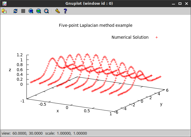
We have used a step size of 0.2 in the above. In order to verify experimentally the second order of convergence of the method we also compute a numerical solution using a step size of 0.1. Using the exact solution $z = e^{-\frac{x^2 + y^2}{2}}$, we compute the maximal error of the numerical solution in both cases. Then we take the ratio of the two errors, which we expect to be close to $2^2$. The output of such a program is shown below and fulfills our expectations.

1D Linear Advection Equation
We consider the 1D linear advection equation of the general form:
- PDE: $\frac{du}{dt} + a \frac{du}{dx} = 0$,
- on the domain: $x\subscript{min} < x < x\subscript{max}$ and $t\subscript{min} < t < t\subscript{max}$,
- with periodic boundary consitions: $u(x\subscript{min},t) = u(x\subscript{max},t)$,
- with initial condition: $u(x,t\subscript{min}) = g(x)$.
The constant $a$ is called the advection velocity. Four different numerical schemes are available in spitzy to solve the advection equation. Those are the Upwind, Leapfrog, Lax-Wendroff and Lax-Friedrichs methods.
Upwind
The Upwind method stems from the approximation of both derivatives with first order finite differences. That is, depending on the sign of the advection velocity $a$, the finite difference representation of the PDE has the form: $$\frac{u\subscript{j}^{n+1} - u\subscript{j}^n}{\Delta t} = -a \frac{u\subscript{j}^{n} - u\subscript{j-1}^n}{\Delta x} + \mathcal{O}(\Delta t, \Delta x), \quad a>0,$$ $$\frac{u\subscript{j}^{n+1} - u\subscript{j}^n}{\Delta t} = -a \frac{u\subscript{j+1}^{n} - u\subscript{j}^n}{\Delta x} + \mathcal{O}(\Delta t, \Delta x), \quad a<0,$$ where $u\subscript{j}^n$ denotes the approximation to $u$ at the $j$th $x$-step and the $n$th time step, and where $\Delta x$ and $\Delta t$ denote the lengths of the corresponding time or space steps.
Consequently, the Upwind scheme is given by the explicit formula: $$u\subscript{j}^{n+1} = u\subscript{j}^n -\frac{a\Delta t}{\Delta x}(u\subscript{j}^n - u\subscript{j-1}^n), \quad a > 0,$$ $$u\subscript{j}^{n+1} = u\subscript{j}^n -\frac{a\Delta t}{\Delta x}(u\subscript{j+1}^n - u\subscript{j}^n), \quad a < 0,$$ depending on the sign of $a$. This is a first-order methods, as is clear by its derivation.
In order to ensure the stability of the method (meaning that the solution will not have exponentially growing modes), the step sizes $\Delta x$ and $\Delta t$ should be chosen such that the so-called CFL (Courant-Friedrichs-Lewy) condition $$\left| \frac{a\Delta t}{\Delta x} \right| \leq 1$$ is satisfied. This can be shown via von Neumann stability analysis. For a rigorous derivation of this and other properties of the Upwind scheme we refer to [Rez11].
Lax-Friedrichs
The Lax-Friedrichs scheme is an explicit first-order method of the form: $$u\subscript{i}^{n+1} = \frac{1}{2}(u\subscript{i+1}^n + u\subscript{i-1}^n) - a\frac{\Delta t}{2\,\Delta x}(u\subscript{i+1}^n - u\subscript{i-1}^n),$$ where, as before, $u\subscript{j}^n$ denotes the approximation to $u$ at the $j$th $x$-step and the $n$th time step, and where $\Delta x$ and $\Delta t$ denote the lengths of the corresponding time or space steps.
It is derived from the following forward-in-time-centered-in-space representation of the PDE: $$\frac{u\subscript{i}^{n+1} - \frac{1}{2}(u\subscript{i+1}^n + u\subscript{i-1}^n)}{\Delta t} + a\frac{u\subscript{i+1}^n - u\subscript{i-1}^n}{2\,\Delta x} = 0.$$
As the Upwind method, in order to ensure the stability of the Lax-Friedrichs method (meaning that the solution will not have exponentially growing modes), the step sizes $\Delta x$ and $\Delta t$ should be chosen such that the so-called CFL (Courant-Friedrichs-Lewy) condition $$\left| \frac{a\Delta t}{\Delta x} \right| \leq 1$$ is satisfied. This can be shown via von Neumann stability analysis. For a rigorous derivation of this and other properties of the Lax-Friedrichs scheme we refer to [Rez11].
Leapfrog
The Lax-Friedrichs scheme, introduced above, is based on a first-order approximation for the time derivative and a second-order approximation for the spatial derivative. Thus, in order to achieve the desired accuracy, $a\Delta t$ needs to be chosen significantly smaller than $\Delta x$, well below the limit imposed by the CFL condition.
The Leapfrog method achieves a second-order accuracy in time by using the centered difference $$\frac{du}{dt} = \frac{u\subscript{j}^{n+1} - u\subscript{j}^{n-1}}{2 \Delta t} + \mathcal{O}(\Delta t^2)$$ in time, and the same centered difference in space as used by the Lax-Friedrichs method.
The resulting Leapfrog scheme, which is second-order in time and space, is $$u\subscript{j}^{n+1} = u\subscript{j}^{n-1} - a\frac{\Delta t}{\Delta x}(u\subscript{j+1}^n - u\subscript{j-1}^n).$$
As the other methods, in order to ensure the stability of the Leapfrog method (meaning that the solution will not have exponentially growing modes), the step sizes $\Delta x$ and $\Delta t$ should be chosen such that the so-called CFL (Courant-Friedrichs-Lewy) condition $$\left| \frac{a\Delta t}{\Delta x} \right| \leq 1$$ is satisfied. This can be shown via von Neumann stability analysis. For a rigorous derivation of this and other properties of the Leapfrog scheme we refer to [Rez11].
Implementation Details
Note that the Leapfrog scheme is a two-level scheme, requiring records of values at time steps $n$ and $n−1$ to get values at time step $n+1$.
Thus, the solution at the second time step must be computed with a different method in order to initialize the Leapfrog scheme. In the current implementation of spitzy the Lax-Wendroff scheme is used to initialize the Leapfrog. Such an implementation of the Leapfrog method yields second-order accuracy as a whole, because both, Lax-Wendroff and Leapfrog, are second-order schemes.
Lax-Wendroff
The Lax-Wendroff scheme is an explicit method which is second-order accurate in time and space. It can be regarded as an extension of the Lax-Friedrichs method. The basic idea in its derivation is to use Lax-Friedrichs evaluations at half steps $t\subscript{n+1/2}$ and $x\subscript{n+1/2}$: $$u\subscript{i+1/2}^{n+1/2} = \frac{1}{2}(u\subscript{i+1}^n + u\subscript{i}^n) - \frac{\Delta t}{2\,\Delta x}( f( u\subscript{i+1}^n ) - f( u\subscript{i}^n ) ),$$ $$u\subscript{i-1/2}^{n+1/2} = \frac{1}{2}(u\subscript{i}^n + u\subscript{i-1}^n) - \frac{\Delta t}{2\,\Delta x}( f( u\subscript{i}^n ) - f( u\subscript{i-1}^n ) ),$$ followed by a Leapfrog "half step": $$u\subscript{i}^{n+1} = u\subscript{i}^n - \frac{\Delta t}{\Delta x} \left( f(u\subscript{i+1/2}^{n+1/2}) - f(u\subscript{i-1/2}^{n+1/2}) \right).$$
Even though the Lax-Wendroff method is technically a two-level scheme, requiring records of values at time steps $n$ and $n+1/2$ to get values at time step $n+1$, it can be algebraically reformulated into the one-level form: $$u\subscript{i}^{n+1} = u\subscript{i}^n -\frac{a\Delta t}{2\Delta x}\left(u\subscript{i+1}^n-u\subscript{i-1}^n\right) + \frac{a^2\Delta t^2}{2\Delta x^2}\left(u\subscript{i+1}^n-2u\subscript{i}^n+u\subscript{i-1}^n\right).$$
As the other methods, in order to ensure the stability of the Lax-Wendroff method (meaning that the solution will not have exponentially growing modes), the step sizes $\Delta x$ and $\Delta t$ should be chosen such that the so-called CFL (Courant-Friedrichs-Lewy) condition $$\left| \frac{a\Delta t}{\Delta x} \right| \leq 1$$ is satisfied. This can be shown via von Neumann stability analysis. For a rigorous derivation of this and other properties of the Lax-Wendroff scheme we refer to [Rez11].
Implementation
The Upwind, Lax-Friedrichs, Leapfrog and Lax-Wendroff methods are implemented in class Advection_eq of the Ruby gem spitzy. The required inputs are the advection speed $a$, the space and time domains (both as intervals represented by arrays of length two in Ruby), the space and time step sizes, and the initial condition as a function of $x$ passed as a Proc object or a block.
An Advection_eq object has various attributes that we can access. In particular, the numerical solution #u is saved as an array of arrays, where the $i$th array contains the values of the solution on the spacial grid at the $i$th time step.
Examples
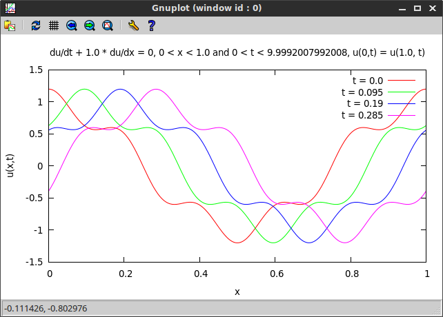
We want to solve the 1D linear advection equation given as:
- PDE: $\frac{du}{dt} + a \frac{du}{dx} = 0$,
- on the domain: $0 < x < 1$ and $0 < t < 10$,
- with periodic boundary conditions: $u(0,t) = u(1, t)$,
- with initial condition: $u(x,0) = \cos(2\pi x) + \frac{1}{5}\cos(10\pi x)$.
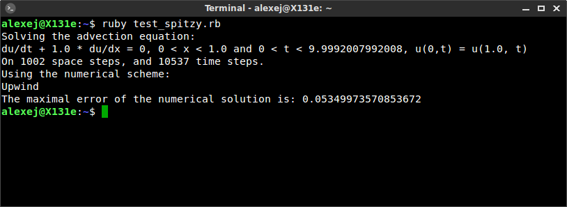
We define and solve this equation using the Upwind scheme with time steps $dt = 0.95/1001$ and spatial steps $dx = 1/1001$ (i.e. on a grid of 1000 equally sized intervals in $x$). Spitzy::AdvectionEq.new lets the user specify the parameters such as length of the space and time steps, time and space domain, the initial condition, etc.
require 'spitzy'
ic = proc { |x| Math::cos(2*Math::PI*x) + 0.2*Math::cos(10*Math::PI*x) }
numsol = Spitzy::AdvectionEq.new(xrange: [0.0,1.0], trange: [0.0, 10.0],
                         dx: 1.0/1001, dt: 0.95/1001, a: 1.0,
                         method: :upwind, &ic)
We can get the equation solved by numsol in form of a character string using the method #equation.
There are four different numerical schemes available to solve the advection equation. Those are the Upwind, Leapfrog, Lax-Wendroff and Lax-Friedrichs methods. We can get which scheme was used by numsol with the attribute reader #method. Similarly we can access the number of $x$-steps #mx and $t$-steps #mt, as well as various other attributes.
Using Fourier methods we compute the exact solution of the PDE to be $\cos(2\pi (x-t)) + 0.2\cos(10\pi (x-t))$. We can use it to check the accuracy of the numerical solution.
Combined, the Ruby code produces the following output (the entire code is given at the end of this post).
Finally, we plot the computed numerical solution at different times using the gnuplot gem (the Ruby code is given below). We use the character string numsol.equation as a header for the plot. We can see a travelling wave as expected.
Conclusions and Future Work
We have introduced all methods currently implemented in the Ruby gem spitzy. We have shown many usage examples, and we have briefly introduced the theoretical basis for each method as well as the underlying differential equations. We have also discussed implementation specifics for all of the numerical schemes. We have seen that some of the methods could not be implemented to be as efficient as they can be, because the numerical linear algebra Ruby gem NMatrix is not as mature yet as other linear algebra libraries for programming languages more commonly used in the scientific community (such as Python or C++). However, the required linear algebra algorithms are currently under active development, and can be incorporated in spitzy in the near future. For example, the #tridiagonal_solve method is implemented already but not merged to the NMatrix project yet (as of 2015/05/07).
Since there is a lack of scientific libraries in general and differential equation solvers in particular for Ruby, spitzy seems to be a project worth extending.
In the immediate future, we need to implement automated test for all numerical methods currently included in spitzy.
Then, more work can be done on the implementation of additional numerical schemes, as well as on the improvement of some of the available methods.
Eventually, it is highly desirable to set up interfaces to publicly available advanced and well-tested numerical codes, written in C or FORTRAN, such as the ones available from the public repositories GAMS or NETLIB.
The author enjoyed it a lot to work on this project, and learned in the process much about open source software development in general, as well as software development in Ruby specifically. Contributions to spitzy are very welcome!
References
- [QSS07] A. Quarteroni, R. Sacco, F. Saleri (2007) Numerical Mathematics, 2nd ed., Texts in Applied Mathematics. Springer.
- [Arn11] D. N. Arnold (2011) Lecture notes on Numerical Analysis of Partial Differential Equations, version of 2011-09-05. Lecture notes MATH 8445 Numerical Analysis of Differential Equations, University of Minnesota. http://www.ima.umn.edu/~arnold//8445.f11/notes.pdf
- [Sha86] L. F. Shampine (1986) Some practical Runge-Kutta formulas. Math. Comput. 46, 173 (January 1986), 135-150. DOI=10.2307/2008219 http://dx.doi.org/10.2307/2008219
- [DP80] J. R. Dormand, P. J. Prince (1980) A family of embedded Runge-Kutta formulae, Journal of Computational and Applied Mathematics 6 (1): 19–26, doi:10.1016/0771-050X(80)90013-3.
- [Rez11] L. Rezzolla (2011) Numerical Methods for the Solution of Partial Differential Equations, Lecture Notes for the COMPSTAR School on Computational Astrophysics, 8-13/02/10, Caen, France. http://www.aei.mpg.de/~rezzolla/lnotes/Evolution_Pdes/evolution_pdes_lnotes.pdf