Quick remark before we get to the theoretical part of this presentation...

Live demos

This lecture contains several live demos. Why?

• DL is largely an empirical research field.
• Sometimes DL in actions seems like magic!
• DL is not my research field — I finally have an excuse to spend some time figuring out the common DL libraries!

Live demos

Main example:

Ultrasound nerve segmentation

• Task: Identify nerve structures in ultrasound images of the neck.
• Needed for effective and accurate insertion of a patient's pain management catheter.

Ultrasound nerve segmentation

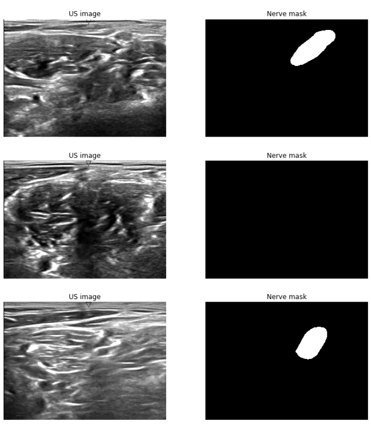
Task: Predict the nerve mask for an input ultrasound image.

5635 training images, 5508 test images.

420×580 resolution.

~47% images don't have a mask.

Data from a $100,000 competition held in 2016: https://www.kaggle.com/c/ultrasound-nerve-segmentation

I will live-execute the following code (more on the hardware & software requirements later):

https://github.com/agisga/ultrasound-nerve-segmentation/blob/master/jupyter/U-net_improved.ipynb

The code borrows from: [1], [2].

Hopefully, by the end of this lecture you will understand all of the components of this deep learning model.

Perceptrons

• Developed in the 50s and 60s by Frank Rosenblatt.
• Inspired by earlier work by Warren McCulloch and Walter Pitts (cf., NAUTILUS. The Man Who Tried to Redeem the World with Logic.).

Weighing multiple input factors to make a decision according to a decision threshold.

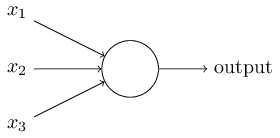
Binary inputs $x_1, x_2, \ldots \in \{0, 1\}$,
and binary output.

Better notation

$$ \begin{eqnarray} \mathbf{x} \mapsto \left\{ \begin{array}{ll} 0 & \mbox{if } \mathbf{w}^T \mathbf{x} + b \leq 0 \\ 1 & \mbox{if } \mathbf{w}^T \mathbf{x} + b > 0 \end{array} \right. \end{eqnarray} $$

• Input vector $\mathbf{x} \in \{0, 1\}^p$,
• Vector of weights $\mathbf{w} \in \mathbb{R}^p$,
• A bias term $b \in \mathbb{R}$,
• An output in $\{0, 1\}$.

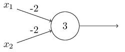
Example: NAND Gate.

That is, 00 $\mapsto$ 1, 01 $\mapsto$ 1, 10 $\mapsto$ 1, 11 $\mapsto$ 0.

(NAND gate is universal for computation. Analogy: a network of perceptrons and a computational circuit.)

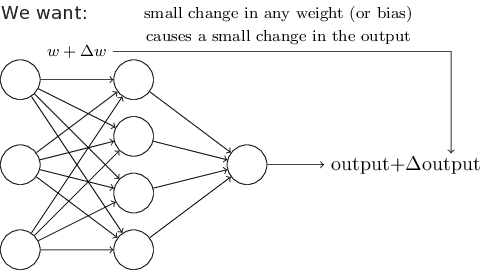
A network of perceptrons

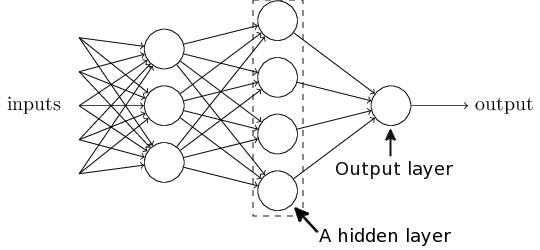
Hidden layer: Making a decision at a more abstract level by weighing up the results of the first layer.

The “Mark 1 perceptron” (Cornell, 1957)

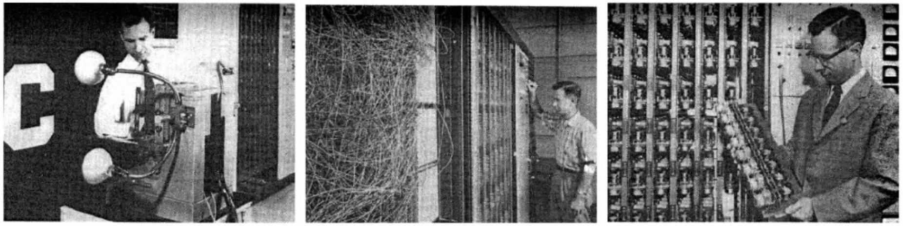
Array of 400 photocells, connected to the “neurons”. The weights ($w_i$) and biases ($b$) are potentiometers.

In 1958 The New York Times reported the perceptron to be “the embryo of an electronic computer that [the Navy] expects will be able to walk, talk, see, write, reproduce itself and be conscious of its existence.” (Mikel Olazaran (1996) A Sociological Study of the Official History of the Perceptrons Controversy)

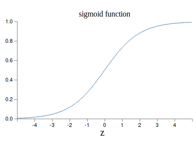
Use the sigmoid function as the activation function.

The sigmoid neuron: $$\mathbf{x} \mapsto \frac{1}{1 + \exp(-\mathbf{w}^T\mathbf{x} - b)}$$

Multilayer perceptron (MLP)

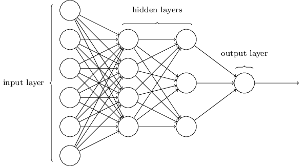
• Made up of sigmoid neurons, not perceptrons — a misnomer?
• Feedforward neural network — no loops allowed.

Universality theorem

Neural networks can be used to approximate any continuous function to any desired precision.

(among other sources, see Chapter 4 in Michael Nielsen's book, or George Cybenko (1989) Approximation by superpositions of a sigmoidal function).

MLP for recognition of handwritten digits

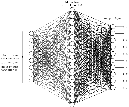
Let's see how well it works in a live demonstration!

Live demonstrations

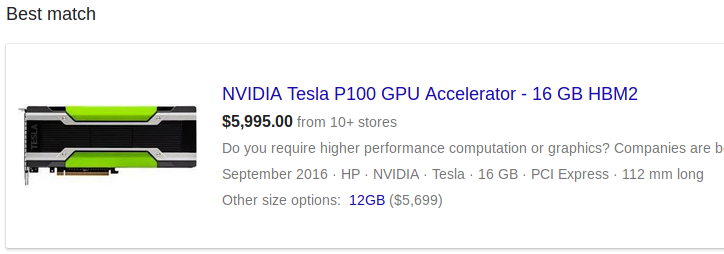
State-of-the-art neural network models require a modern GPU (or GPUs).

In this talk I use the following setup on a Google Cloud virtual machine.

Instructions to reproduce the same exact setup can be found at https://github.com/agisga/coding_notes/blob/master/google_cloud.md.

Components:

• NVIDIA Tesla P100 GPU rented on Google Cloud (about $1.19 per hour), and GPU drivers on linux
  
• CUDA and cuDNN libraries for numerical computing on the GPU.
• TensorFlow, with Keras as frontend.
• Python, SciPy, NumPy, Jupyter Notebook, ...

Classification of handwritten digits

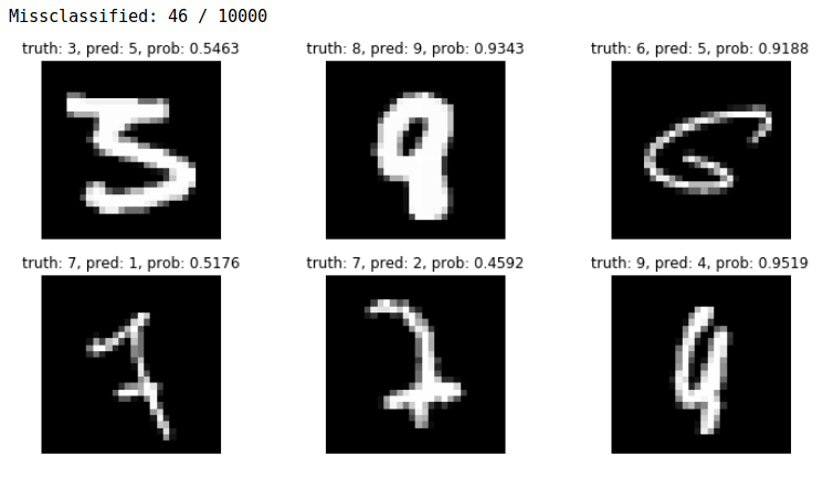
I will execute the following code:

https://github.com/agisga/coding_notes/blob/master/Keras/MNIST_functional_API.ipynb

Stochastic gradient descent (SGD)

How do we find the optimal weights and biases?

Cost function: $$C = \frac{1}{2n} \sum\subscript{i=1}^n \lVert y(\mathbf{x}_i) - a(\mathbf{x}_i) \rVert_2^2,$$ where $a(\mathbf{x}_i)$ is the output of the NN and $y(\mathbf{x}_i)$ is the desired output for the input $\mathbf{x}_i$.

Gradient descent

• $ \begin{bmatrix} \mathbf{w} + \Delta \mathbf{w} \\ b + \Delta b \end{bmatrix} \leadsto C + \Delta C. $
• $\Delta C \approx \nabla C \cdot \begin{bmatrix} \Delta \mathbf{w} \\ \Delta b \end{bmatrix}$.
• We want: $\Delta C < 0$.
• Update: $ \begin{bmatrix} \mathbf{w} \\ b \end{bmatrix} \gets \begin{bmatrix} \mathbf{w} \\ b \end{bmatrix} - \eta \nabla C. $
• $\eta > 0$ is called the learning rate.

Stochastic gradient descent (SGD)

$C = \frac{1}{2n} \sum\subscript{i=1}^n \lVert y(\mathbf{x}_i) - a(\mathbf{x}_i) \rVert_2^2 = \frac{1}{n} \sum\subscript{i=1}^n C_i$,

where $C_i := (y(\mathbf{x}_i) - a(\mathbf{x}_i))^2 / 2$.

Randomly choose a subset $\mathbf{x}\subscript{i_1}, \ldots, \mathbf{x}\subscript{i_m}$ of size $m\ll n$.

Then, $\nabla C \approx \frac{1}{m} \sum\subscript{j=1}^m \nabla C\subscript{i_j}$,

The set $\{\mathbf{x}\subscript{i_1}, \ldots, \mathbf{x}\subscript{i_m}\}$ is called a mini-batch.

Stochastic gradient descent (SGD)

1. Pick a mini-batch size $m \ll n$.
2. Randomly (without replacement) choose a mini-batch $\mathbf{x}\subscript{i_1}, \ldots, \mathbf{x}\subscript{i_m}$.
3. Update all weights and biases: $$ \begin{bmatrix} \mathbf{w} \\ b \end{bmatrix} \gets \begin{bmatrix} \mathbf{w} \\ b \end{bmatrix} - \frac{\eta}{m} \sum\subscript{j=1}^m \nabla C\subscript{i_j}. $$
4. Repeat 2-3.
5. An epoch is completed, when every input $\mathbf{x}_i$ has been used.

Stochastic gradient descent (SGD)

Now we only need to figure out how to differentiate $C\subscript{i_j}$ with respect to every weight and every bias in the neural network...

The backpropagation algorithm

• 1986 paper by Rumelhart, Hinton, and Williams.
• The “workhorse” of deep learning.

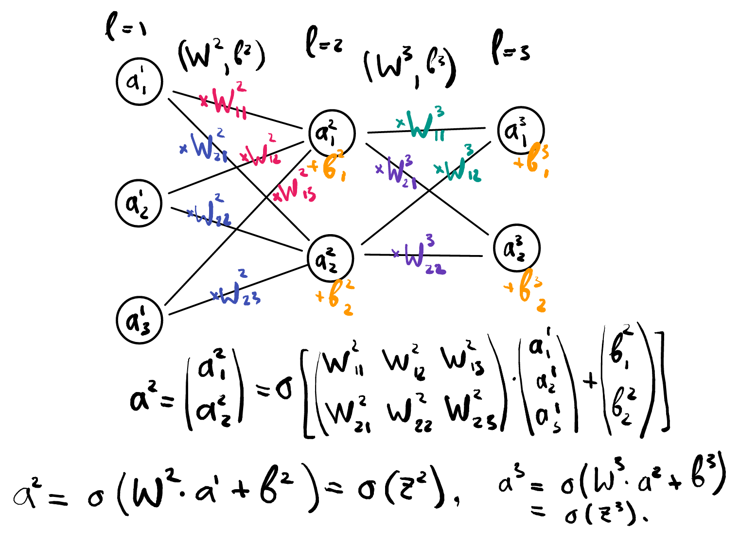
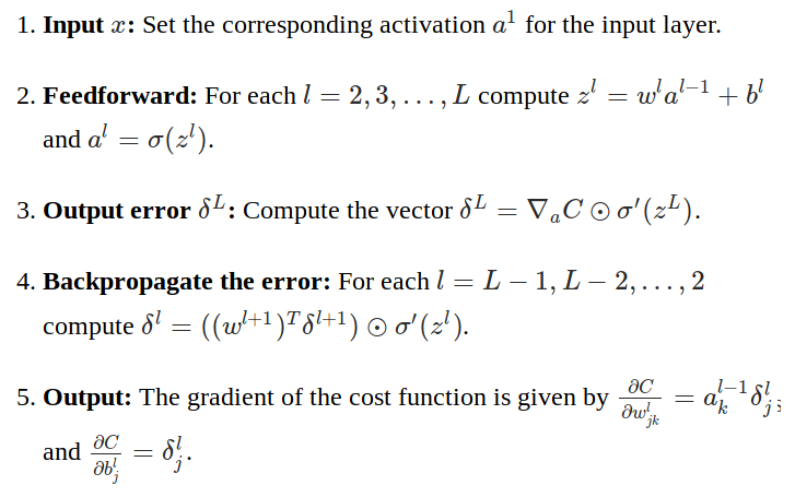
More better notation

• Layers $l = 1, 2, \ldots, L$.
• $\mathbf{a}^1 :=$ input layer (as a vector).
• $\mathbf{a}^l :=$ activations of layer $l$ (as a vector).
• $W^l :=$ matrix of weights at layer $l$.
• $\mathbf{b}^l :=$ vector of biases at layer $l$.
• $\mathbf{z}^l := W^l \mathbf{a}^{l-1} + \mathbf{b}^l$.

$$\Rightarrow \mathbf{a}^l = \sigma(W^l \mathbf{a}^{l-1} + \mathbf{b}^l) = \sigma(\mathbf{z}^l)$$

Chain rule!

Layer L (last layer): $$ \begin{eqnarray} \frac{\partial C}{\partial W\subscript{ij}^L} &=& \nabla\subscript{\mathbf{a}^L} C \cdot \frac{\partial \sigma(\mathbf{z}^L)}{\partial \mathbf{z}^L} \cdot \frac{\partial \mathbf{z}^L}{\partial W\subscript{ij}^L} \nonumber \\ &=:& \delta^L \cdot \frac{\partial \mathbf{z}^L}{\partial W\subscript{ij}^L} = \delta^L \cdot \mathbf{a}_j^{L-1} \nonumber \end{eqnarray} $$

Layer L-1: $$ \begin{eqnarray} \frac{\partial C}{\partial W\subscript{ij}^{L-1}} &=& \nabla\subscript{\mathbf{a}^L} C \cdot \frac{\partial \sigma(\mathbf{z}^L)}{\partial \mathbf{z}^L} \cdot \frac{\partial \mathbf{z}^L}{\partial \mathbf{z}^{L-1}} \cdot \frac{\partial \mathbf{z}^{L-1}}{\partial W\subscript{ij}^{L-1}} \nonumber \\ &=& \delta^L \cdot W^L \cdot \frac{\partial \sigma(\mathbf{z}^{L-1})}{\partial \mathbf{z}^{L-1}} \cdot \frac{\partial \mathbf{z}^{L-1}}{\partial W\subscript{ij}^{L-1}} \nonumber \\ &=:& \delta^{L-1} \cdot \frac{\partial \mathbf{z}^{L-1}}{\partial W\subscript{ij}^{L-1}} \nonumber = \delta^{L-1} \cdot \mathbf{a}_j^{L-2} \nonumber \end{eqnarray} $$

Likewise, any other layer $l$: $\frac{\partial C}{\partial W\subscript{ij}^{l}} = \delta^{l} \cdot \mathbf{a}_j^{l-1}$,
where $\delta^{l}$ is determined by $\delta^{l+1}$, $W^{l+1}$, and $\partial \sigma(\mathbf{z}^{l}) / \partial \mathbf{z}^{l}$.

The backpropagation algorithm

Backpropagation — Aside:

https://www.axios.com/artificial-intelligence-pioneer-says-we-need-to-start-over-1513305524-f619efbd-9db0-4947-a9b2-7a4c310a28fe.html

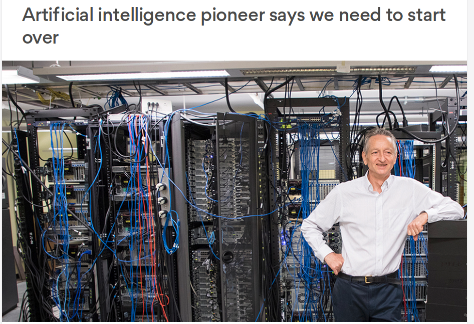
Backpropagation — Aside:

Hinton (...) is now “deeply suspicious” of back-propagation (...). “My view is throw it all away and start again,” he said.
(...)
“Max Planck said, ‘Science progresses one funeral at a time.’ The future depends on some graduate student who is deeply suspicious of everything I have said.”

Improving the way NN work

There are a lot of techniques, tricks, and best practices (some based on theory, some on empirical trial and error). Here is a small selection.

Least squares loss: Learning slowdown b/c $\nabla C$ depends on $\sigma^\prime(z)$ ($\approx 0$ for $|z| > 5$).

A better choice of cost fnct.

Categorical cross-entropy: $$ C = -\frac{1}{n} \sum_x [y \ln(a) + (1-y) \ln(1-a)]. $$

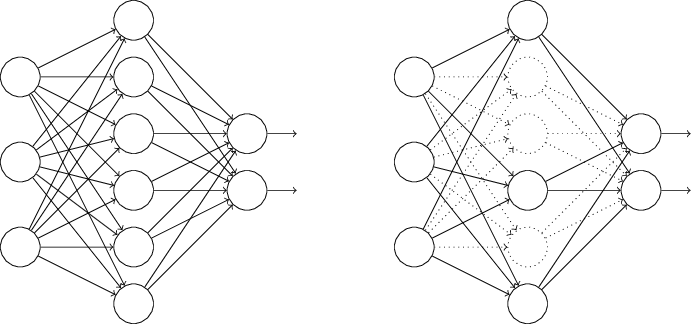
Regularization

Reduce over-fitting to the training data.

• L2: minimize $C + \frac{\lambda}{2n}\sum_w w^2$.
• L1: minimize $C + \frac{\lambda}{n}\sum_w |w|$.
• Dropout: Within every iteration of backprop, randomly and temporarily delete some neurons.

Variations of SGD

• Hessian technique
• Momentum-based GD
• Many more: An overview of gradient descent optimization algorithms (a blog post by Sebastian Ruder)

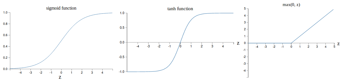
Activation functions

• Sigmoid: $\frac{1}{1 + \exp(-\mathbf{w}^T\mathbf{x} - b)}$
• Hyperbolic tan: $\mathrm{tanh}(\mathbf{w}^T\mathbf{x} + b)$
• Rectifier linear unit (ReLU): $\max(0, \mathbf{w}^T \mathbf{x} + b)$.
• Softmax. E.g., in MNIST last layer: $a_j^L = \frac{\exp(z_j^L)}{\sum_{k = 0}^9 \exp(z_k^L)}$ can be interpreted as "probability" that input image shows digit $j$.

Let's try these techniques on the handwritten digit recognition example.

Backpropagation — the vanishing gradient problem in deep NN

(unrelated to Hinton's remarks on a previous slide)

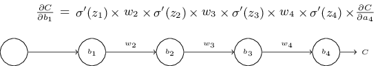
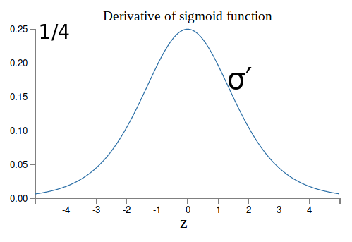
With standard initialization $|w_j|<1$, as so, $|w_j \sigma^\prime(z_j)| < 1/4$. $\Rightarrow$ Vanishing gradient in the earlier layers of a deep model $\Rightarrow$ The earlier layers "learn" much slower than later layers.

Likewise: exploding gradient when all $|w_j \sigma^\prime(z_j)| \gg 1$.

Deep Learning

Convolutional neural network

Deep convolutional network is the most widely used type of deep nearal network.

Modern CNN: LeCun, Bottou, Bengio, Haffner (1998).

Convolution

Each neuron in the hidden layer is connected to only $5 \times 5 = 25$ input activations (pixels).

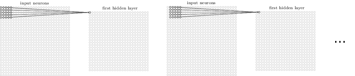
• The 25 weights and the bias parameter are shared (i.e., the same for each hidden neuron). $\Rightarrow$ Drastic reduction in the number of parameters.
• Each neuron looks for the same "feature", just at a different location.

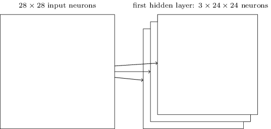
Convolutional layer

A complete convolutional layer uses several convolutional filters to produce several different feature maps.

Pooling layers

Most common: max-pooling

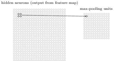
Other options: L2-pooling, average pooling.

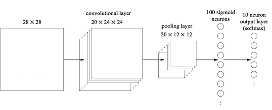
Convolutional neural network

Putting it all together

Many types of convolutions

Vincent Dumoulin, Francesco Visin - A guide to convolution arithmetic for deep learning

Animations source: https://github.com/vdumoulin/conv_arithmetic

Convolutional neural network

Let's try it on the handwritten digit recognition example.

Deep learning

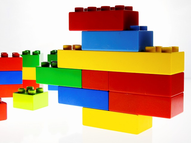
Modular nature.

Many building blocks.

Segmentation DL architectures — U-net

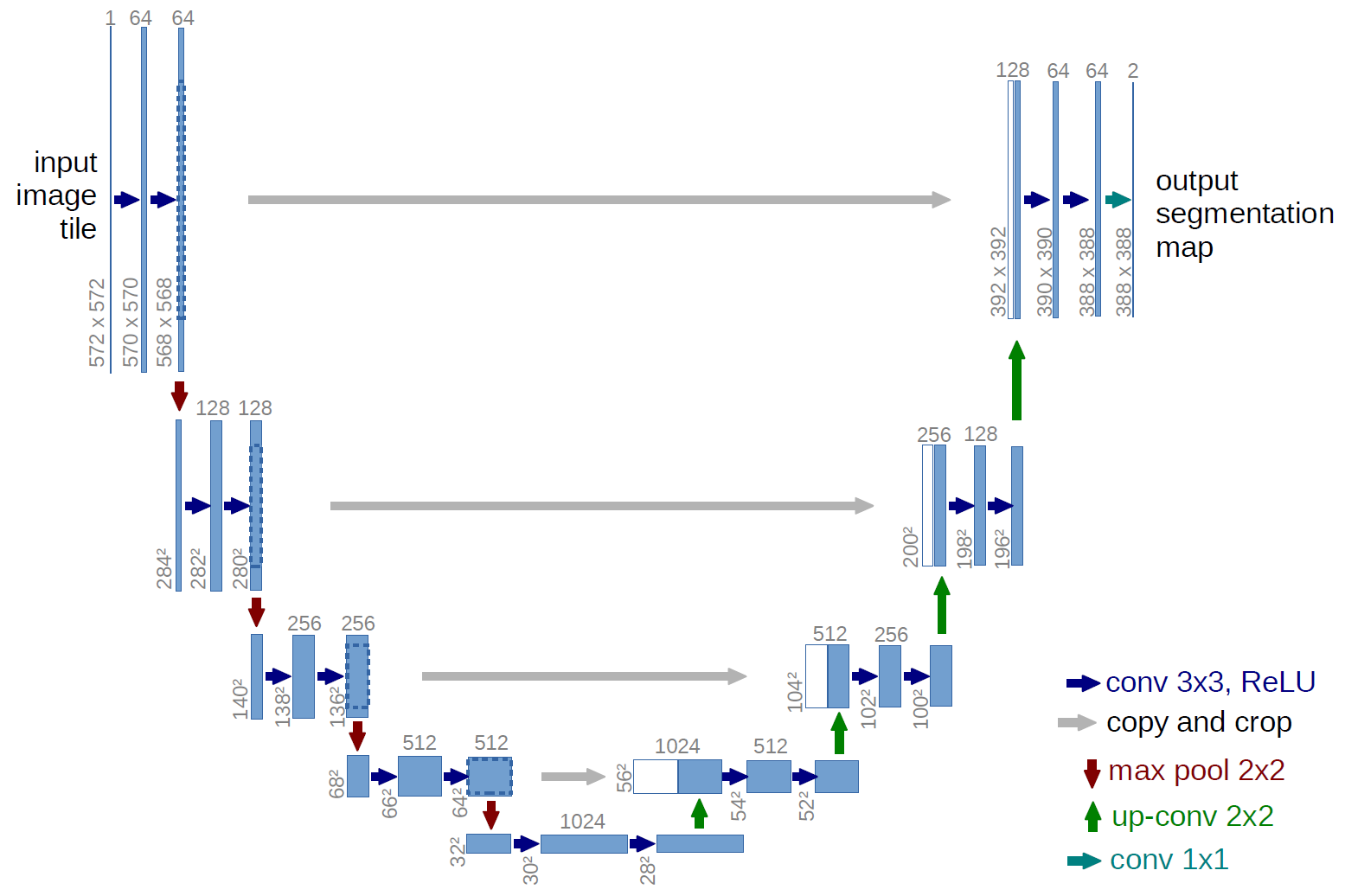
Ronneberger, Fischer, Brox. 2015. "U-Net: Convolutional Networks for Biomedical Image Segmentation." Medical Image Computing and Computer-Assisted Intervention (MICCAI), Springer, LNCS, Vol.9351: 234--241.

Back to the ultrasound image segmentation example.