Basic usage of the R package grpSLOPE
Introduction
Group SLOPE (gSLOPE) is a penalized linear regression method that is used for adaptive selection of groups of significant predictors in a high-dimensional linear model. A unique property of the Group SLOPE method is that it offers group false discovery rate (gFDR) control (i.e., control of the expected proportion of irrelevant groups among the total number of groups selected by Group SLOPE). A detailed description of the method can be found in D. Brzyski, A. Gossmann, W. Su, and M. Bogdan (2019) “Group SLOPE — adaptive selection of groups of predictors” Journal of the American Statistical Association (or the 2016 arXiv preprint).
Group SLOPE is implemented in the R package grpSLOPE. As an introduction to the R package, in the following we will walk through a basic usage demonstration. First, we will simulate some data, before we feed it into grpSLOPE, and subsequently examine the output.
Data generation
We simulate a $500 \times 500$ SNP-data-like model matrix.
set.seed(17082016)

p     <- 500
probs <- runif(p, 0.1, 0.5)
probs <- t(probs) %x% matrix(1,p,2)
X0    <- matrix(rbinom(2*p*p, 1, probs), p, 2*p)
X     <- X0 %*% (diag(p) %x% matrix(1,2,1))
For example, the upper left $10 \times 10$ corner of $X$ looks as follows.
1 1 0 1 0 0 1 2 0 0
0 0 1 1 0 0 1 1 1 0
1 0 1 1 0 0 1 0 0 0
1 0 0 0 1 0 0 0 2 2
1 0 0 1 1 1 0 0 1 1
0 1 0 0 0 0 2 1 2 2
0 0 0 0 1 2 0 0 2 0
2 0 0 0 0 0 0 1 0 2
1 0 1 0 0 1 0 1 1 1
0 0 1 0 0 0 0 0 1 1
Note: In fact, with the default settings, the Group SLOPE method is guaranteed to control gFDR only when applied to a data matrix, where the columns corresponding to different groups of predictors are nearly uncorrelated. The relevant theoretical results can be found in Brzyski et. al. (2016). Only for the brevity of exposition we neither check for nor enforce low between-group correlations in this example.
We divide the 500 predictor variables into 100 groups of sizes ranging from 3 to 7.
group <- c(rep(1:20, each=3),
           rep(21:40, each=4),
           rep(41:60, each=5),
           rep(61:80, each=6),
           rep(81:100, each=7))
group <- paste0("grp", group)
str(group)
## chr [1:500] "grp1" "grp1" "grp1" "grp2" "grp2" ...For further usage we keep additional information about the grouping structure of predictors, such as the total number of groups and the group sizes.
# this generates a list containing a vector of indices for each group:
group.id <- grpSLOPE::getGroupID(group)
# this extracts the total number of groups:
n.group <- length(group.id)
# this vector collects the sizes of every group of predictors:
group.length <- sapply(group.id, FUN=length)
# this vector collects the group names:
group.names <- names(group.id)
In order to simulate a response variable, we randomly select 10 groups to be truly significant.
ind.relevant <- sort(sample(1:n.group, 10)) # indices of relevant groupsThe randomly selected truly significant groups are:
grp4 grp13 grp22 grp34 grp35 grp59 grp65 grp68 grp72 grp78
Then we generate the vector of regression coefficients, by sampling effect sizes for the significant groups from the Uniform(0,1) distribution.
b <- rep(0, p)
for (j in ind.relevant) {
  b[group.id[[j]]] <- runif(group.length[j])
}
Finally, we generate the response vector according to a linear model with i.i.d. $\mathcal{N}(0, 1)$ noise terms.
y <- X %*% b + rnorm(p)Fitting the Group SLOPE model
We fit the Group SLOPE model to the simulated data. The function argument fdr signifies the target group-wise false discovery rate (gFDR) of the variable selection procedure.
library(grpSLOPE)

model <- grpSLOPE(X=X, y=y, group=group, fdr=0.1)
Model fit results
The resulting object model of class “grpSLOPE” contains a lot of information about the resulting Group SLOPE model. Some of these parameters are shown below.
- Groups that were selected as significant by the Group SLOPE method.
model$selected
    ##  [1] "grp4"  "grp11" "grp13" "grp22" "grp34" "grp35" "grp59" "grp65"
    ##  [9] "grp68" "grp72" "grp78"
Notice that the model has correctly identified all significant groups, and additionally has falsely reported the group “grp11” as significant.
- The estimated noise level $\hat{\sigma}$ (true $\sigma$ is equal to one).
sigma(model) # or equivalently: model$sigma
## [1] 0.9886372
- The regression coefficients, which can be displayed either on the normalized scale (i.e., the scale corresponding to the normalized versions of $X$ and $y$, on which all the parameter estimates are computed internally),
    # the first 13 coefficient estimates
    coef(model)[1:13]
    ##   grp1_1   grp1_2   grp1_3   grp2_1   grp2_2   grp2_3   grp3_1
    ## 0.000000 0.000000 0.000000 0.000000 0.000000 0.000000 0.000000
    ##   grp3_2   grp3_3   grp4_1   grp4_2   grp4_3   grp5_1
    ## 0.000000 0.000000 4.127673 1.613667 5.232564 0.000000
or on the original scale of $X$ and $y$,
    # intercept and the first 13 coefficient estimates
    coef(model, scaled = FALSE)[1:14]
    ## (Intercept)      grp1_1      grp1_2      grp1_3      grp2_1
    ##   3.8190431   0.0000000   0.0000000   0.0000000   0.0000000
    ##      grp2_2      grp2_3      grp3_1      grp3_2      grp3_3
    ##   0.0000000   0.0000000   0.0000000   0.0000000   0.0000000
    ##      grp4_1      grp4_2      grp4_3      grp5_1
    ##   0.2727357   0.1000815   0.4077402   0.0000000
(notice that the coefficients are named corresponding to the given grouping structure). As expected from a penalized regression method, we observe some shrinkage, when we compare the above to the true parameters.
    # true first 13 coefficients
    b[1:13]
    ##  [1] 0.0000000 0.0000000 0.0000000 0.0000000 0.0000000 0.0000000
    ##  [7] 0.0000000 0.0000000 0.0000000 0.3677210 0.1713692 0.6425599
    ## [13] 0.0000000
- It might also be interesting to plot the first few elements of the regularizing sequence $\lambda$ used by the Group SLOPE method for the given inputs.
plot(model$lambda[1:10], xlab = "Index", ylab = "Lambda", type="l")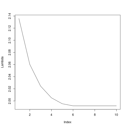
We can further check the performance of the method by computing the resulting group false discovery proportion (gFDP) and power.
true.relevant <- group.names[ind.relevant]
truepos       <- intersect(model$selected, true.relevant)

n.truepos  <- length(truepos)
n.selected <- length(model$selected)
n.falsepos <- n.selected - n.truepos

gFDP <- n.falsepos / max(1, n.selected)
pow <- n.truepos / length(true.relevant)

print(paste("gFDP =", gFDP))
[1] “gFDP = 0.0909090909090909”
print(paste("Power =", pow))[1] “Power = 1”
We see that the method indeed did not exceed the target gFDR, while maintaining a high power.
Lambda sequences
Multiple ways to select the regularizing sequence $\lambda$ are available.
If a group structure with little correlation between groups can be assumed (i.e., groups in the standardized model matrix are nearly orthogonal), then we suggest to use the sequence “corrected”, which is the default.
The $\lambda$ sequences “mean” and “max” can be used together with the options orthogonalize = FALSE and normalize = FALSE, when the columns of the model matrix are exactly orthogonal to each other (“max” is more conservative, giving exact gFDR control only when all groups have the same size, and otherwise resulting in a lower gFDR than the target level).
Alternatively, any non-increasing sequence of appropriate length can be utilized. However, we do not recommend to use any other $\lambda$ sequences unless you really know what you are doing.
References
-
Bogdan, M., van den Berg, E., Sabatti, C., Su, W., and Candès, E. J. (2015), SLOPE — Adaptive Variable Selection via Convex Optimization. The Annals of Applied Statistics, vol. 9, no. 3, p. 1103.
-
D. Brzyski, A. Gossmann, W. Su, and M. Bogdan (2019) Group SLOPE — adaptive selection of groups of predictors. Journal of the American Statistical Association 114 (525): 419–33.
-
Gossmann, A., Cao, S., and Wang, Y.-P. (2015). Identification of Significant Genetic Variants via SLOPE, and Its Extension to Group SLOPE. In Proceedings of the 6th ACM Conference on Bioinformatics, Computational Biology and Health Informatics, BCB ’15 (pp. 232–240). New York, NY, USA: ACM.